Reinforcement Learning Notes
Reinforcement Learning
-When we think about the nature of learning, we think about interaction
-Reinforcement learning focuses on a computational approach to goal-directed learning from interaction
1.1 Reinforcement Learning
-The learner is not specifically told which actions to take, but learns through trial and error in addition to delayed reward
- these two features distinguish RL from other ML
-Formally, RL uses ideas from dynamical systems theory, specifically, "incompletely-known Markov decision processes"
- learning agent must sense environment, must be able to take action and must have goals
-RL contrasts with supervised learning in that SL seeks to obtain generalizability from historical labels
- RL meanwhile is trying to learn from interaction and not necessarily from charted territory
-unsupervised learning is also distinguished by the fact that its trying to find representations in the data and it has nothing to do with a reward signal
-Therefore, we consider RL to be a third paradigm of ML
-One of the challenges of RL is the trade-off between exploration and exploitation
- to maximize reward, it can exploit past behaviors its deemed rewarding
- but to find those behaviors in the first place, it has to explore and possibly lose reward
- The catch is that the task cannot be accomplished by either one exclusively
- The exploration-exploitation dilemna remains unsolved
-RL is part of a swing of the pendulum in AI research towards discovery of principles, as opposed to rules based
1.3 Elements of Reinforcement Learning
-The 4 main elements of an RL system are: a policy, a reward signal, a value function and optionally, a model of the environment
a policy defines the agent's way of behaving.
- Its a mapping from perceived states of the environment to actions to be taken in those states (in psychology, called associations and from their perspective is the basis for learning)
- may be as simple as a lookup or as complicated as a search process
a reward signal defines the goal of the RL system.
- The reward is that which the system is trying to maximize and is the primary basis for altering policy
- it is more immediate term
a value function specifies what is good in the long-term
- The specifies the total amount of reward which can be expected in the long-term
But rewards are primary, and values are predictions of rewards. Without rewards there could be no values.
- However, when making and evaluating decision, we use values since they provide the most reward to us over time
- Values are difficult to determine, while rewards are a given
- Value estimation is one of the most important things to have been progressed in RL research in the last 60 years
a model of the environment allows inferences to be made about how the environment will behave
- e.g. given a state and an action, the model might predict next state and reward
- models are used for planning and are not in all RL systems
1.4 Limitations and Scope
-RL relies on the concept of "state", as input to the policy and value function
- essentially it conveys to the agent some sense of how the environment is
- We will focus mainly on estimating value functions (but you don't need this to solve RL problems)
1.5 An Extetnded Example: Tic-Tac-Toe
-assuming you play against an imperfect player, how can we construct a player which will learn the opponent's imperfections and maximize its chance of winning?
classicial optimization techniques (dynamic programming) require complete specification of opponent, including the probabilities with which the opponent makes each move
essentially, we can learn a model of the opponent's behavior from experience to get these probabilities and then apply dynamic programming (many RL methods do this)
or, using a value function.
- We would set of a table of numbers, each representing the probabilities of winning from each state of the tic-tac-toe board
- this estimate is the state's value
- set all initial values of the states to 0.5
- then play many games against the opponent, greedily selecting the moves (moving to states with greatest value) and occasionally randomly selecting another move to explore
- then we "back up" value of states so that earlier states are nudged closer in value to later states

1.6 Summary
-RL is a computational approach to understanding and automating goal-directed learning and decision making
- it distinguishes itself from other computational approaches in its interaction-based learning and the lack of need of direct supervision or model of environment
- its fundamentally based on Markov decision processes
- the concepts of value and value function are key to most RL methods
1.7 History of RL
-Early History of RL contains two threads which eventually merged:
- Psychology of animal learning
- Optimal control and dynamic programming
-They merged around a third thread known as temporal difference methods and modern RL began in 80s
-Optimal control thread centers around Bellman equation and the class of methods used to solve this equation known as dynamic programming
- Bellman also introduced the discrete stochastic version of this problem known as Markov decision processes
-trial-and-error learning was first coherently captured b Edward Thorndike
The "Law of Effect": Behaviors which produce a satisfying effect are more likely to occur when the situation presents itself again and behaviors which produce a painful effect are less likely to occur for that situation
Later learning automata had an influence on trial-and-error learning (k-armed bandit)
-temporal difference learning has its origins in animal psychology with secondary reinforcers
- It was brought together with optimal control with Chris Watkin's Q-learning
Multi-armed Bandits
-The most important difference between RL and SL is that RL evaluates the actions of the bot rather than instructing
- SL indicates the correct action to be taken, independent of the action
- RL indicates how good the action was
-To begin, we study the evaluative aspect of RL in a simplified setting which does not involve learning to act in more than one situation (nonassociative setting)
2.1 A k-armed Bandit Problem
-You are faced repeatedly with a choice among k different options, or actions
- After each choice, you receive a numerical reward chosen from a stationary PDF that depends on the action you selected
- Your objective is to maximize the expected total reward over some time period, for example 1000 time steps
- This problem is named after the analogy to the slot machine (the "one-armed bandit"), except that it has k levers
-Each of the k actions has an expected reward, and we call this the value of the action:
$$ q_{*}(a) \coloneqq \mathbf{E}[R_{t}|A_{t}=a] $$Where $q_{*}(a)$ is the expected reqward, given that action $a$ is selected. $R_{t}$ is the reward and $A_{t}$ is the action
-To estimate this, we would need a joint distribution of $R_{t}$ and $A_{t}$
-If you maintain estimates of the value of actions, then at any time step, there is at least one action whose estimated value is the greatest
- Taking this action would be the greedy action and when you do, we say that you are exploiting you current knowledge of the values of the actions
- If you choice one of the nongreedy actions, we say that you are exploring (this might lead to a greater reward in the long term)
- Balancing exploitation and exploration is a difficult task but leads to a more optimal solution than just exploiting
2.2 Action-value Methods
-estimate the values of actions and use the estimates to make action selection decisions
-Simply average the rewards seen when particular action was taken:
$$ Q_{t}(a) \coloneqq \frac{\text{sum of rewards when $a$ taken prior to t}}{\text{number of times $a$ taken prior to t}} $$$$ Q_{t}(a) = \frac{\sum_{i=1}^{t-1}R_{i}\cdot \bm{1}_{A_i=a}}{\sum_{i=1}^{t-1} \bm{1}_{A_{i}=a}} $$as t goes to infinity, $Q_{t}(a)$ converges to $q_{*}(a)$.
-This is not necessarily the best way to estimate the value!
-Simplest action selection rule is to select the action with the highest estimated value (greedy):
$$A_{t} \coloneqq \underset{a}{\mathrm{argmax}}Q_{t}(a) $$-Slight mod of this is behaving greedy most of the time, but every once in a while, with small probability $\epsilon$, select randomly from all actions
- we call these methods $\epsilon-greedy$ methods
- advantage here is that in the limit of $t \rightarrow \infty$, you sample all of the actions infinitely thus ensuring $Q_{t}(a)$ converges to $q_{*}(a)$
2.3 The 10-armed Testbed
-To assess greedy vs $\epsilon-greedy$, we analyze a set of 2000 randomly generated $k$-armed bandit problems with $k=10$
-The true values, $q_{*}(a)$, were selected from a normal distribution. The reward, $R_{t}, for each action is also a normal distribution but with mean $q{*}(A{t})$
-For any learning method, we can measure its performance for 1000 steps, and this constitutes 1 run
- then repeat this procedure 2000 times (effectively a different bandit problem each time)

-What you then see is that the greedy algorithm performs better initially but plateaus at a lower reward
-The slight exploration allows discovery of that higher expected reward of 1.5

-For noisier rewards (more variance), the $\epsilon-greedy$ methods would fare even better than the greedy model
-In the deterministic case of no variance, the greedy would quickly find the solution
- But if the values of the actions were not stationary, it would be worthwhile to explore to make sure one of the other actions have not changed to become the better one
2.4 Incremental Implementation
-To calculate action values in a computationally efficient manner, we will consider a simple derivation
-Let $R_{i}$ denote the reward received after the $ith$ selection of this action and let $Q_{n}$ denote the estimate of its action value after having been selected $n-1$ time:
$$ Q_{n} \coloneqq \frac{R_{1} + R_{2} + ... + R_{n-1}}{n-1} $$-We don't need to perform this computation over and over again
-It can be shown that, given $Q_{n}$ and the $nth$ reward $R_{n}$:
$$ Q_{n+1} = Q_{n} + \frac{1}{n}[R_{n} - Q_{n}] $$so you only need memory for $Q_{n}$ and $n$
-This update rule thats the form that comes up frequently:
$$ \text{New Estimate} \leftarrow \text{Old Estimate} + \text{Step Size}[\text{Target - Old Estimate}] $$-In this case the target is the nth reward and $\text{Target - Old Estimate}$ is an error estimate
-Note that the $\text{Step Size}$ gets smaller with increasing actions of this type taken
-Below is the pseudo code for the bandit algorithm

2.5 Tracking a Nonstationary Problem
-When reward probabilities change over time, it makes sense to give more weight to recent rewards
-It's common to modify the step size parameter to be constant for nonstationary reward pdfs
-It can be shown that in this case, $Q_{n+1}$ becomes a weighted average of the past rewards:
$$Q_{n+1} = (1 - \alpha)^{n}Q_{1} + \sum_{i=1}^{n}\alpha(1-\alpha)^{n-i}R_{i} $$-This turns out to be an exponentially weighted average!
-For the constant $\alpha$ case, the value function estimates actually never converge for large $n$, but this is what we want in nonstationary problems!
2.6 Optimistic Initial Values
-The methods above depend on the initial action-value estimates, $Q_{1}(a)
This is known as a biased estimate in statistics
For the sample-average method, the bias disappears once all actions have been selected at least once
But for consant $\alpha$ they persist
-An initial bias in the value function, lets say 5 in the k-armed bandit problem is overly optimistic
- But this over-optimism causes the algorithm to initially explore as it is disappointed in the rewards it is receiving
- These optimistic initial values are good for encouraging exploration in stationary problems but not so with nonstationary since the exploration is only temporary in the beginning of the run
- In addition, the sample-average technique also represents a bias towards the beginning of time since it weighs all subsequent rewards equally
2.7 Upper-Confidence-Bound Action Selection
-In the $\epsilon-greedy$ algorithm, if we could give preference to those actions which have some uncertainty and are close to being maximal
-you can capture this with the following:
$$A_{t} \coloneqq \underset{a}{\mathrm{argmax}}[Q_{t}(a) + c\sqrt{\frac{lnt}{N_{t}(a)}}] $$-this upper confidence bound action selection takes into account the uncertainty in the estimate of $a$'s value
-The quantity being index maxed is essesntially the upper bound of that action's value
-As $N_{t}(a)$ increases, i.e. you've observed that action more, the uncertainty in it's value decreases
Finite Markov Decision Processes
-This essentially is the main problem we try to solve
-There is evaluative feedback, as with the bandits, but now there is an associative aspect (choosing different actions in different situations)
- Actions influence not just immediate rewards, but also subsequent situations (or states)
- Hence MDPs involve delayed reward and the need to tradeoff immediate and delayed reward
-With k-armed bandits, we estimated $q_{*}(a)$ of each action $a$, while with MDPs, we estimate $q_{*}(s,a)$ or each action $a$ in each state $s$
- or we estimate the value $v_{*}(s)$ of each state given optimal action selections
-MDPs are a mathematically idealized form of the RL problem
3.1 The Agent-Environment Interface
-The learner and decision maker is called the agent
-The thing it interacts with is called the environment
-The agent and environment interact continually where the agent is selecting actions and the environment is responding to these actions by presenting new situations
- The environment also gives rise to rewards, which the agent seeks to maximize over time with its actions

-The agent and environment interact at discrete time steps $t=0,1,2,3,...$
-At each time step, the agent receives a representation of the environment's state, $S_t \in S$ and from that, selects an action, $A_t \in A(s)$
One time step later, the agent receives a reward $R_{t+1} \in R$ and finds itself in a new state $S_{t+1}$
The trajectory looks like this:
$$ S_0, A_0, R_0, S_1, A_1, R_1, S_2, A_2, R_2, ... $$
-In a finite MDP, the sets of states, actions, and rewards ($S, A, R$) all have a finite number of elements
-In this case, the random variables $R_t$ and $S_t$ have well defined discrete probability distributions dependent only on the preceding state and action:
$$ p(s',r|s,a) \coloneqq Pr(S_t=s', R_t=r|S_{t-1}=s,A_{t-1}=a) $$-In a Markov decision process, the probabilities given by $p$ completely characterize the environment's dynamics
The probability of each $S_t$ and $R_t$ only depend on the immediately preceding state and action and not at all on earlier states and actions
The state must include all aspects of the past agent-environment that make a difference for the future (Markov property)
-Can compute the state-transition probabilities:
$$ p(s'|s,a) \coloneqq Pr(S_t=s'|S_{t-1}=s,A_{t-1}=a) = \sum_{r \in R}p(s',r|s,a) $$-Can compute the expected rewards for state-action pairs
$$ r(s,a) \coloneqq \mathbf{E}[R_{t}|S_{t-1}=s,A_{t-1}=a] = \sum_{r \in R}r\sum_{s' \in S}p(s',r|s,a) $$-The general rule is that whatever cannot be changed by agent is considered part of its environment
-But we always consider the reward computation to be external to the agent because it defined the task facing the agent and is beyond its ability to change arbitrarily
- agent might know everything of environment (rubik's cube) but still face a difficult RL problem
- The agent-environment boundary represents the limit of the agent's absolute control, not of its knowledge
-Any problem of goal-directed behavior can be reduced to 3 signals pass back and forth between the agent and the environment:
- one signal represents the choice made by the agent (the actions)
- another signal represents the basis on which the choices are made (the states)
- and the other signal defines the agent's goals (the rewards)
3.2 Goals and Rewards
-Reward Hypothesis
- All that we mean by goals and purposes is the maximization of the expected value of the cumulative sum of a recieved scalar signal
-The reward signal is your way of communicating to the robot what you want it to achieve, not how you want it achieved
3.3 Returns and Episodes
-We seek to maximize the expected return, where the return, denoted $G_{t}$, is defined as some function of the reward sequence
-In the simplest case, the return is the sum of the rewards:
$$ G_{t} \coloneqq R_{t+1} + R_{t+2} + R_{t+3} + ... + R_{T} $$Where $T$ is the final time step. This makes sense in applications where there is a notion of a final time step.
-When the agent-environment interaction breaks naturally into subsequences, called episodes, such as plays of a game
- each episode ends in a special state called the terminal state
- the next episode begins independently of how the previous one ended (episodic tasks)
- Some interactions do not break down into episodes (continuing tasks) (above formulation of return doesn't work then since it blows up)
-We additionally need the concept of discounting, where the agent tries to select actions so that the sum of the discounted rewards it recieves over the future is maximized:
$$ G_{t} \coloneqq R_{t+1} + \gamma R_{t+2} + \gamma^2 R_{t+2} + ... = \sum_{k=0}^{\infty} \gamma^k R_{t+k+1}$$Where $\gamma$ is the discount rate, ranges from $0\le\gamma\le1$. As $\gamma$ approaches 1, the return objective takes future rewards into account more strongly (it becomes more farsighted)
-This discounting also makes the infinite sum finite (Geometric series)!
3.5 Policies and Value Functions
-All RL algorithms involve estimating value functions
these are functions of states (or state-action pairs) that estimate how good it is for the agent to be in a given state (in terms of expected return)
the rewards an agent can expect to receive in the future depend on what actions it will take
- therefore, value functions are defined w.r.t. particular ways of acting (policies)
-The value function of a state $s$ under policy $\pi$, denoted $v_{\pi}(s)$ is the expected return when starting in $s$ and following $\pi$ thereafter. For MDPs:
$$ v_{\pi}(s) \coloneqq \mathbf{E}_{\pi}[G_{t}|S_{t}=s] = \mathbf{E}_{\pi}[\sum_{k=0}^{\infty}\gamma^{k}R_{t+k+1}|S_{t}=s]\text{ for all } s \in S $$We call $v_{\pi}$ the state-value function for policy $\pi$
-Also, we define the value of taking action $a$ in state $s$ under policy $\pi$, denoted $q_{\pi}(s,a)$ as the expected return starting from $s$, taking the action $a$, and thereafter following policy $\pi$:
$$ q_{\pi}(s,a) \coloneqq \mathbf{E}_{\pi}[G_{t}|S_{t}=s, A_{t}=a] = \mathbf{E}_{\pi}[\sum_{k=0}^{\infty}\gamma^{k}R_{t+k+1}|S_{t}=s, A_{t}=a] $$and we call $q_{\pi}$ the action value function for policy $\pi$
-in practice, one can estimate $v_{\pi}$ and $q_{\pi}$ from experience
- if we store averages for each action taken and for each state (Monte Carlo methods)
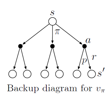
-A fundamental property of value functions throughout RL is that they satisfy a recursive relationship
-For any policy $\pi$ and any state $s$, it can be shown that the following holds between the value of $s$ and the value of its possible successor states:
$$ v_{\pi}(s) = \sum_{a}\pi(a|s)\sum_{s',r}p(s',r|s,a)[r+\gamma v_{\pi}(s')]\text{ for all } s \in S $$Where $\pi(a|s)$ is the probability that $A_{t}=a$ if $S_{t}=s$ (the policy). The is the Bellman Equation for $v_{\pi}$.
-The Bellman equation expresses a relationship between the value of a state and the values of its successor states
The Bellman equation averages over all the possibilities, weighting each by its probability of occurring
It states that the value of the start state must equal the discounted value of the expected next state, plus the reward expected along the way
3.6 Optimal Policies and Optimal Value Functions
-Solving an RL task means finding a policy which achieves a lot of reward over the long run
-The optimal policies have value functions greater than the other policies
- They share the same state-value function, called the optimal state-value function
- They also share the same optimal action-value function
-We can then show that the Bellman optimality equation is:
$$ v_{*}(s) = \max_{a}\sum_{s',r}p(s',r|s,a)[r+\gamma v_{*}(s')] $$-For finite MDPs, the Bellman optimality equation has a unique solution
its a actually a system of $n$ nonlinear equations in $n$ unknowns
you just need the transition probabilities, and the rewards associated with those transitions
-One can easily select the optimal policy based off a greedy selection of the action which maximizes the optimality equation
term greedy is used in CS to describe selections of alternatives based only off of local considerations
greedy in RL describes selecting actions only based on short term consequences
but if you greedily use $v_{*}$ you're fine because the quantity already takes into account the long term
using $q_{*}$ is even easier because you don't even need to do the one-step-ahead search. Just find the action which maximizes it
-The issue with explicitly solving the Bellman optimality equations is that it is akin to an exhaustive search and is rarely useful
we need to know the dynamics of the environment to use Bellman
we need plenty of computational resources
we need the Markov property
-In practice, some combinatination of the above 3 assumptions are not met
- e.g. backgammon has $10^20$ states and would take a modern computer thousands of years to solve the Bellman equation for $v_{*}$
-Many RL methods can be seen as approximating solving the Bellman optimality equation
3.7 Optimality and Approximation
-The optimal policies typically can only be generation with extreme computational cost
- A critical aspect of the problem facing the agent is always the computational power available to it
-Also, a large amount of memory is required to build up approximations of value functions, policies and models
- Sometimes the state space is so large, we cannot fit this information into a table
-So we do approximations and approximations in the sense that we might be ok with suboptimal decisions in low probability state spaces
3.8 Summary
-RL is about learning from interaction how to behave in order to achieve a goal
-The RL agent and its environment interact over discrete time steps
-The specification of their interface defines a task:
- The actions are the choices made by the agent
- The states are the basis for taking the actions
- The rewards are the basis for evaluating the choices
-A policy is a stochastic rule by which the agent selects actions as a function of states
-When this problem described above is formulated with well defined transition probabilities, it is a Markov Decision Process (MDP)
A finite MDP is where you have a finite state, action and reward set
much of current RL theory is restricted to finite MLPs
-The return is the function of future rewards
undiscounted version is appropriate for episodic tasks
discounted version appropriate for continuing tasks
-A policy's value functions assigns to each state, or state-action pair, the expected return from that state, or state-action pair, given that the agent uses the policy
The optimal value functions assign to each state, or state-action pair, the largest expected return achievable by any policy
A policy whose values function are optimal is an optimal policy
Can solve the Bellman optimality equations for the optimal value functions, from which an optimal policy can be determined with ease
-Limitations on computations and memory mean we must approximate
- solving Bellman is an ideal!
- Andrew Barto in video with Sutton: "RL is memorized context-sensitive search"
Dynamic Programming
Dynamic programming refers to a collection of algorithms that can be used to compute optimal policies given a perfect model of the environment like with MDPs
Classical DP algs are of limited utility in RL because of assumption of perfect model and computational expense
- but its an important theoretical foundation for understanding later modern methods
Key idea of DP, and of RL generally, is the use of value functions to organize and structure the search for good policies
4.1 Policy Evaluation (Prediction)
-iterative policy evaluation is when you use the Bellman equations to update the value functions at each step
- in theory, it should converge to the optimal value function

4.2 Policy Improvement
-we compute the value function for a policy to help find better policies
-how do we know when to diverge from policy?
-one can consider the action-value function, where you select an action then follow the policy
key idea is whether $q_{\pi}(s,a)$ is greater than $v_{\pi}(s)$
- then we would know to always take action $a$ when $s$ is encountered, and this would be a new policy
Gen any pair of deterministic policies $\pi$ and $\pi'$, the policy improvement theorem states that if:
Then $\pi'$ must be as good as or better than $\pi$. It must obtain greater than or equal expected return from all states:
$$v_{\pi'} \ge v_{\pi}(s)$$Its a natural extension to consider changes to all states and to all possible actions,selecting at each state the action which maximizes the action-value function.
The greed policy, $\pi'$ is then:
The process of making a new policy that improves on the original policy, by making it greedy w.r.t. to value function of original policy is called policy improvement
4.3 Policy Iteration
-once a policy $\pi$ has been improved using $v_{\pi}$ to yield a better policy $\pi'$, we can then compute $v_{\pi'}$ and improve it again to yield an even better $\pi''$

where $E$ is the policy evaluation and $I$ is the policy improvement
-Since the finite MDP has only a finite number of policies, this process must converge to an optimal policy and optimal value function in a finite number of iterations

4.4 Value Iteration
-stopping policy evaluation after just one sweep is known as value iteration

-Kelly Criterion example!

4.6 Generalized Policy Iteration
-generalized policy iteration refers to simply letting policy evaluation and policy improvement interact, independent of the granularity of the two processes
- they can be viewed as both competing and interacting
4.7 Efficiency of Dynamic Programming
-DP might not be practical for very large problems but it finds an optimal policy in polynomial time
exponentially faster than any direct search
sometimes LP might be better but as the number of states increases, DP is the only feasible way
DP thought to be of limited applicability because of curse of dimensionality (number of states grows exponentially with the number of state variables)
- but these are inherent difficulties of the problem, not of DP as a solution method