The Data Scientist's Odyssey

Discrete Time Markov Chains¶

A discrete-time random process, {${X_m,m=0,1,2,…}$}, is a sequence of random variables that are observed at different time steps. In the simplest case where the $X_m$'s are independent, the analysis of this process is straightforward. However, in many real-life situations, the $X_m$'s are not independent and we need to develop models where the value of $X_m$ depends on the previous values. One such model is a Markov chain which is typically the shorthand used for what is the discrete time Markov chain.

In a Markov chain, $X_{m+1}$ depends on $X_m$, but given $X_m$, it does not depend on the other previous values $X_0, X_1, \ldots, X_{m-1}$. This means that conditioned on $X_m$, the random variable $X_{m+1}$ is independent of the random variables $X_0, X_1, \ldots, X_{m-1}$. Another way to look at it is, determination of future states only depends on the current state and not the past states. This Markov property is sometimes called memorylessness. In practice, Markov chains are used to model the evolution of states in probabilistic systems. For example, if we are modeling a queue at a bank, the number of people in the queue can be defined as the state of the system.

Formal Definition¶

Let us define a random process {${X_n,n=0,1,2,\ldots}$}, where the random variables' ranges, $R_{X_i} = S \subseteq \{0,1,2,\ldots\}$, are discrete. For any positive integer $m$ and possible states $i_0, i_1, ..., i_{m}$, we say that the process is in state $i_m$ at time $m$ if $X_m = i_m$. Formally, this process is a Markov chain if $$P(X_{m+1}=j|X_m=i,X_{m-1}=i_{m-1},\ldots,X_0=i_0) = P(X_{m+1}=j|X_m=i)$$ for all $m,j,i,i_0,i_1,\ldots i_{m-1}$. This is known as the Markov Property. The numbers $P(X_{m+1}=j|X_m=i)$ are called the transition probabilities and they do not depend on time. Thus, we can define a transition probability matrix:

$$p_{ij} = P(X_{m+1}=j|X_m=i)$$

Here, $p_{ij}$ is the probability of transitioning from state $i$ to state $j$.

In addition, we also have $p_{ij} = P(X_1=j|X_0=i) = P(X_2=j|X_1=i) = P(X_3=j|X_2=i) = \ldots$. This means that if the process is in state $i$, it will next make a transition to state $j$ with probability $p_{ij}$, independent of what particular time step we find ourselves at.

Code Example¶

We can write Python code to simulate a Markov chain. The following code simulates a Markov chain with 12 states. The simulation can then be plotted to visualize the evolution of the chain.

Or with fewer states:

Distribution Evolution¶

Markov processes have cool and simple properties which allow us to directly calculate the evolution of the probability distribution through time, using basic linear algebra! How cool is that? Let's see how this works.

Consider a state space $X_n \in S = \{0,1,2,\ldots,r\}$, where $r$ is the number of states. The initial distribution, $\pi^{(0)}$, is defined by the row vector:

$$\pi^{(0)} = [P(X_0=0), P(X_0=1), \ldots, P(X_0=r)]$$

The distribution at the next time step can be determined using the Law of Total Probability:

$$P(X_1=j) = \sum_{i=0}^r P(X_1=j|X_{0}=i)P(X_{0}=i)$$

of course we recognize this as a matrix multiplication:

$$ P(X_1=j) = \sum_{i=0}^r \pi^{(0)}_i p_{ij}$$$$\pi^{(1)} = \pi^{(0)}p$$

and in general:

$$\pi^{(n)} = \pi^{(n-1)}p$$$$\pi^{(n)} = \pi^{(0)}p^n$$

In practice, if we know the probability distribution at time step 0, we can calculate the probability distribution at time step 1. This is done by multiplying the initial distribution by the transition probability matrix. We can then calculate the distribution at time step 2 by multiplying the distribution at time step 1 by the transition probability matrix. This process can be repeated to calculate the distribution at any time step as long as you know the initial distribution and the transition probability matrix.

Now what if we ask another question. What is the probability of going from state $i$ to state $j$ in $2$ steps? Intuitively, you're now asking about a transition between states when a certain time as elapsed. Once again, we can use the law of total probability by summing over all possible states at time step 1:

$$P(X_2=j|X_0=i) = \sum_{k=0}^r P(X_2=j|X_{1}=k,X_{0}=i)P(X_{1}=k|X_{0}=i)$$

by the markov property:

$$P(X_2=j|X_1=k,X_0=i) = P(X_2=j|X_1=k)$$

so

$$P(X_2=j|X_0=i) = \sum_{k=0}^r P(X_2=j|X_{1}=k)P(X_{1}=k|X_{0}=i)$$$$P(X_2=j|X_0=i) = \sum_{k=0}^r p_{kj}p_{ik}$$

this is just matrix multiplication:

$$P(X_2=j|X_0=i) = p^2$$

We can extend this result to what is known as the Chapman-Kolmogorov equation:

$$P(X_m=j|X_n=i) = p^{(m+n)}_{ij} = p^np^m$$

Absorption Probabilities, Mean Hitting Times and Mean Return Times¶

In order to understand some critical concepts in Markov chains such as mean hitting time and mean return time, we need to examine Markov chains from a diagrammatic perspective and state some definitions.

One of the most basic definitions is accessibility. A state $j$ is accessible from state $i$ if there is a path from $i$ to $j$, written as $i \rightarrow j$. Mathematically, this means that for some $n$, there is a finite transition probability from $i$ to $j$:

$$p_{ij}^{(n)} > 0$$

Furthermore, two states are said to communicate if they are accessible to each other. This means that there is a path from $i$ to $j$ and a path from $j$ to $i$. Mathematically, this means that for some $n$, there is a finite transition probability from $j$ to $i$ and a finite transition probability from $i$ to $j$:

$$p_{ij}^{(n)} > 0 \text{ and } p_{ji}^{(n)} > 0$$

A Markov chain can be partitioned into a set of communicating classes where each class is a set of states that communicate with each other. Lets look at a Markov diagram below to visualize this.

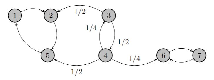
In the diagram above, states 1,2, and 5 are a communicating class, states 3 and 4 are a communicating class, and states 6 and 7 are a communicating class.

You'll notice that there are certain states that are transient (meaning there is a chance you won't return) and other states which are recurrent (meaning you will definitely return). In the diagram above, states 1,2, and 5 are recurrent and states 3 and 4 are transient.

Formally, a state is recurrent if:

$$p_{ii}^{(n)} = 1 \text{ for some } n \gt 0$$

and it is transient if:

$$p_{ii}^{(n)} < 1 \text{ for all } n \gt 0$$

In addition, the number of times a recurrent state is visited after leaving it is infinite. It can be shown that the number of times a transient state is visited after leaving it follows a Geometric random variable. These definitions extend to classes in that if two states are in the same class, then they are both recurrent or both transient.

We also have the concept of periodicity where you can only come back to a certain state after a certain number of steps with a greatest common divisor. In other words, a class has periodicity $k$ if $k$ is the greatest common divisor or all integers $n>0$ for which $p_{ii}^{(n)} > 0$

For an irreducible Markov chain (all states communicate), the chain is aperiodic if there is a self transition. It can also be classified as aperiodic if the period of it is 1.

We can now talk about absorption probabilities, mean hitting times, and mean return times.

Consider the following Markov chain:

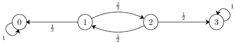
Another concept with Markov chains is the concept of absorbing states where, essentially, once you enter you never leave. 0 and 3 in the above diagram are absorbing states. Now, to find the probability of absorption into 3, given an initial state, we would like to calculate the probability.

We once again use the law of total probability, and specifically the law of total probability for conditional probability:

$$ P(A|C) = \sum_{i=1}^r P(A|B_i, C)P(B_i|C)$$

where $r$ is the number of outcomes over the set of disjoint events $B_i$. Lets define $a_i$ to be the absorption into state 3, given you start in state $i$. Then we can write:

$$a_i = P(\text{absorption into 0} | X_{0}=i) $$$$a_i = \sum_{k=0}^r P(\text{absorption into 0} | X_{1}=k, X_{0}=i) P(X_{1}=k|X_{0}=i) $$

Then by Markov property:

$$a_i = \sum_{k=0}^r P(\text{absorption into 0} | X_{1}=k) P(X_{1}=k|X_{0}=i) $$

so

$$a_i = \sum_{k=0}^r a_i p_{ik} $$

Remembering that we are trying to solve for the absorption probability from state $3$, we have the set of equations:

$$ a_0 = 0 $$$$ a_1 = \frac{1}{3}b_0 + \frac{2}{3}b_2 $$$$ a_2 = \frac{1}{2}b_1 + \frac{1}{2}b_3 $$$$ a_3 = 1 $$

two equations and two unknowns mean we can solve for $a_1$ and $a_2$!

Now we can move on to the mean hitting time which is just the expected time to hit a certain set of states. The same procedure follows, where we sum the probabilities to transition to a certain state multiplied by its mean hitting time. The equation is completely analogous. Formally, $t_{i}$ is defined as the mean hitting time to a set of states beginning at state $i$:

$$ t_{i} = E[T|X_{0}=i] $$

where $T$ is the first time the chain visits the target state. In practice this conditional expectation value can be calculated as:

$$ t_{i} = 1 + \sum_{k} t_{k}p_{ik} $$

To get the mean return time, we just apply this same equation to the situation where we start in the state we are attempting to calculate the mean return time for.

Distributions in the Limit¶

How can we find out if a Markov chain converges to a stationary distribution, and what that distribution is? Assuming that the chain is irreducible and aperiodic, we can use a very simple and intuitive equation. If the chain is in steady-state, then we should get the same distribution when evolving forward one time step via matrix multiplication against the transition probability matrix:

$$ \pi = \pi P $$

where $\pi$ is the stationary distribution. So, the solution to this equation is the stationary distribution, if one exists.

Summary¶

In this article, we have learned about the fundamental stochastic process known as the Markov chain. In this process, the Markov property is its essential feature, which essentially says that future states are independent of the past given the present. A key quantifier of the Markov chain is its transition probability matrix, which is a matrix that describes the probability of transitioning from one state to another. We learned how to simulate a basic Markov chain in Python and saw how the increasing size of the state space leads to a noisier signal. We also know now how to evolve the probability distribution of the states forward in time using simple matrix multiplication agains the transition probability matrix. We learned about Markov chain diagrams and how to classify the states of a Markov chain as transient or recurrent. We then discussed the concept of absorption and how to calculate the probability of absorption into a certain state, in addition to the mean hitting and return times. Finally, we learned how to find the stationary distribution of a Markov chain which involves the solution to a seemingly simple equation. These set of concepts are a pretty good place to start when it comes to stochastic processes and reinforcement learning via Markov decision processes.

Sources¶

Introduction. (n.d.). Www.probabilitycourse.com. Retrieved January 25, 2023, from https://www.probabilitycourse.com/chapter11/11_2_1_introduction.php

‌Markov Chains | Brilliant Math & Science Wiki. (n.d.). Brilliant.org. https://brilliant.org/wiki/markov-chains/#:~:text=A%20Markov%20chain%20is%20a

Using the Law of Total Probability with Recursion. (n.d.). Www.probabilitycourse.com. Retrieved March 26, 2023, from https://www.probabilitycourse.com/chapter11/11_2_5_using_the_law_of_total_probability_with_recursion.php